
Why understanding the limits of a production forecast matters as much as improving its accuracy.
By Bryan Monk, P.Eng. | Founder, MISIM Modelling
A mining feasibility study brings years of technical work together into an investment case. Mine plans, equipment, processing capacity, capital and operating assumptions become a production schedule, then a valuation.
The result is a forecast.
Sensitivity analysis then tests what happens to value when key assumptions change. Production is varied by 5% or 10%, alongside price, capital and operating cost.
That's useful. It shows which assumptions move value the most.
But it leaves an important question unanswered.
How well do we actually understand the range of production outcomes the operation might achieve?
A sensitivity can calculate the value of producing 10% less. It can't tell us how likely that is, what operating conditions would cause it, or whether a larger shortfall is plausible.
In our short explainer on variability and uncertainty, and in an earlier post on transforming the mine value chain, we separated two sources of production risk: how the operation varies around an assumed basis, and whether that basis is right.
This post takes the next step. What do we do when we can't confidently say how likely the alternative bases are? And how do we choose between investments when we're asked to maximize production and minimize cost at the same time?
That's where deep uncertainty comes in.
1. Not all uncertainty is the same
Mining operations vary. Equipment fails, maintenance takes assets offline, material properties change, crews and schedules shift. Even with every assumption held constant, repeated simulations give different annual results.
This is operating variability. It refines the engineering: equipment sizing, storage and operating strategy.
A different problem arises when we question the assumptions themselves. Will the selected equipment achieve the availability we assumed? Will the workforce reach the productivity in the plan? Will the ore behave as the testwork suggests?
Running the same model thousands of times with the same assumed availability doesn't answer those questions.
Operating variability describes different outcomes under an assumed basis. Basis uncertainty concerns whether that basis is correct.
Basis uncertainty also comes in degrees. Walker, Lempert and Kwakkel describe five levels, from a clear enough future to the unknown. Translated to a mining study:
| Level | What we know | Mining example | Treatment |
|---|---|---|---|
| 1 | A clear enough future | Hoist skip payload, conveyor design rate | A single value |
| 2 | Alternatives with known probabilities | Failure and repair behaviour from a comparable operating fleet | Distributions and simulation |
| 3 | Alternatives we can rank, but not quantify | Ore hardness domains where testwork favours one case | Weighted scenarios, with the weights stated as judgment |
| 4 | Plausible alternatives we can't rank | Development rates or labour productivity for a new mining method in a new jurisdiction | Explore across them and test decisions for robustness |
| 5 | What we haven't thought of | A failure mode no one anticipated | Monitoring, flexibility and adaptive plans |
Levels 4 and 5 are what the decision-making literature calls deep uncertainty: situations where decision-makers can't confidently determine, or can't agree on, how the system links decisions to outcomes, the probabilities of key inputs, or which outcomes matter most. These ideas are developed in Decision Making under Deep Uncertainty (Marchau and colleagues, 2019) and discussed in Max Reddel's Model-Based Policy Analysis under Deep Uncertainty (2023).
Most studies sit across several levels at once. A brownfield expansion may be mostly Level 2. A greenfield project with an unproven mining method may have its most important assumptions at Level 4.
The right treatment differs by level. Where evidence supports likelihoods, alternative bases can be weighted and combined into one production distribution, as our explainer shows. Where it doesn't, the weights are themselves an assumption, and a single combined distribution can hide that.
The difficulty isn't only that the forecast might be wrong. It's that we may not know enough to say how likely the alternatives are.
2. Precise answers from uncertain assumptions
Modern simulation can represent an integrated operation in considerable detail: equipment reliability, schedules, maintenance, shared resources, material flows and storage. That matters, because integrated performance can't be inferred from the capacities of individual parts.
But model detail and confidence are different things.
A simulation may run thousands of replications and produce a smooth distribution with well-defined percentiles. Those percentiles may be statistically precise estimates of what the model generates. They're still conditional on the assumptions used.
An apparently precise P50 can coexist with substantial uncertainty about what production the project should expect.
Reddel names two common habits in predictive modelling: collapsing an uncertain range into a single number, and varying uncertain inputs slightly, running a few cases and averaging the results. Both are familiar in mining studies. The first is the study basis. The second is often how alternative assumptions get folded back into one answer.
The answer isn't to abandon probabilistic modelling. Where credible probability information exists, use it. The point is to be clear about which probabilities are supported by evidence, which are conditional on assumptions, and which can't yet be justified.
A carefully constructed range of plausible outcomes is sometimes more useful than a distribution whose precision exceeds the evidence behind it.
3. From predicting production to evaluating decisions
Project analysis usually follows a familiar sequence: set the expected conditions, forecast production and value, test sensitivities, then choose the option that performs best under the expected case.
The decision literature calls this predict-then-act. It works well when the important assumptions are well understood. It breaks down when credible alternative assumptions point to different investments.
Decision-making under deep uncertainty (DMDU) turns the sequence around. It starts with candidate decisions and stress tests each one across many plausible futures. In the U.S. Climate Resilience Toolkit's introduction to DMDU, Rob Lempert and Michelle Miro describe this as seeking confidence in a decision rather than in a specific model.
The question changes from:
"What investment is optimal under our expected assumptions?"
to:
"Which investment performs acceptably across the conditions we might face?"
An option with the highest NPV under one operating basis may perform poorly if that basis is wrong. Another may produce slightly less value under the study basis but stay attractive across a much wider range of conditions. Which is preferable depends on the evidence behind the scenarios and the consequences of underperforming.
That choice should be examined explicitly, not buried in a single forecast.
4. A mining example: where should additional capital go?
Consider an operating mine evaluating several investments: more haul trucks, a crusher or plant upgrade, expanded stockpile capacity, and improvements to outbound rail.
Each has an engineering rationale. More trucks improve ore delivery. A plant upgrade raises throughput. More storage buffers interruptions. Better rail service relieves product constraints.
Conventional analysis estimates the incremental production and return of each proposal under the current operating plan.
But future performance depends on conditions that remain uncertain. Ore hardness may change as mining advances. Truck productivity may differ from plan. Rail performance may change.
Under one set of conditions, trucks deliver the most benefit. Under another, the plant governs production and the trucks add little. Under a third, rail limits what can be sold.
These effects interact. Adding capacity in one area moves the constraint somewhere else, as we discussed in the value chain post.
The decision also isn't one investment. It's a combination: two more trucks or four, with or without the crusher upgrade, with or without more storage, with or without the rail improvements. A handful of options quickly becomes dozens of combinations, each with its own capital cost and production outcome.
An integrated model can evaluate each combination across plausible operating conditions. That reveals what must be true for an investment to create value.
5. Maximize production, minimize cost
Project teams are often asked to do both. Usually they can't. Beyond a point, more production costs more capital.
Plot each investment combination by its incremental capital and the production it delivers. Some combinations are clearly worse than others: another combination delivers at least as much production for less capital. These are dominated, and they can be set aside without debating commodity price, discount rate or risk appetite.
What remains is the Pareto front: the combinations where you can't gain production without spending more, or save capital without losing production. Every point on the front is a defensible choice. Moving along it trades capital for production.
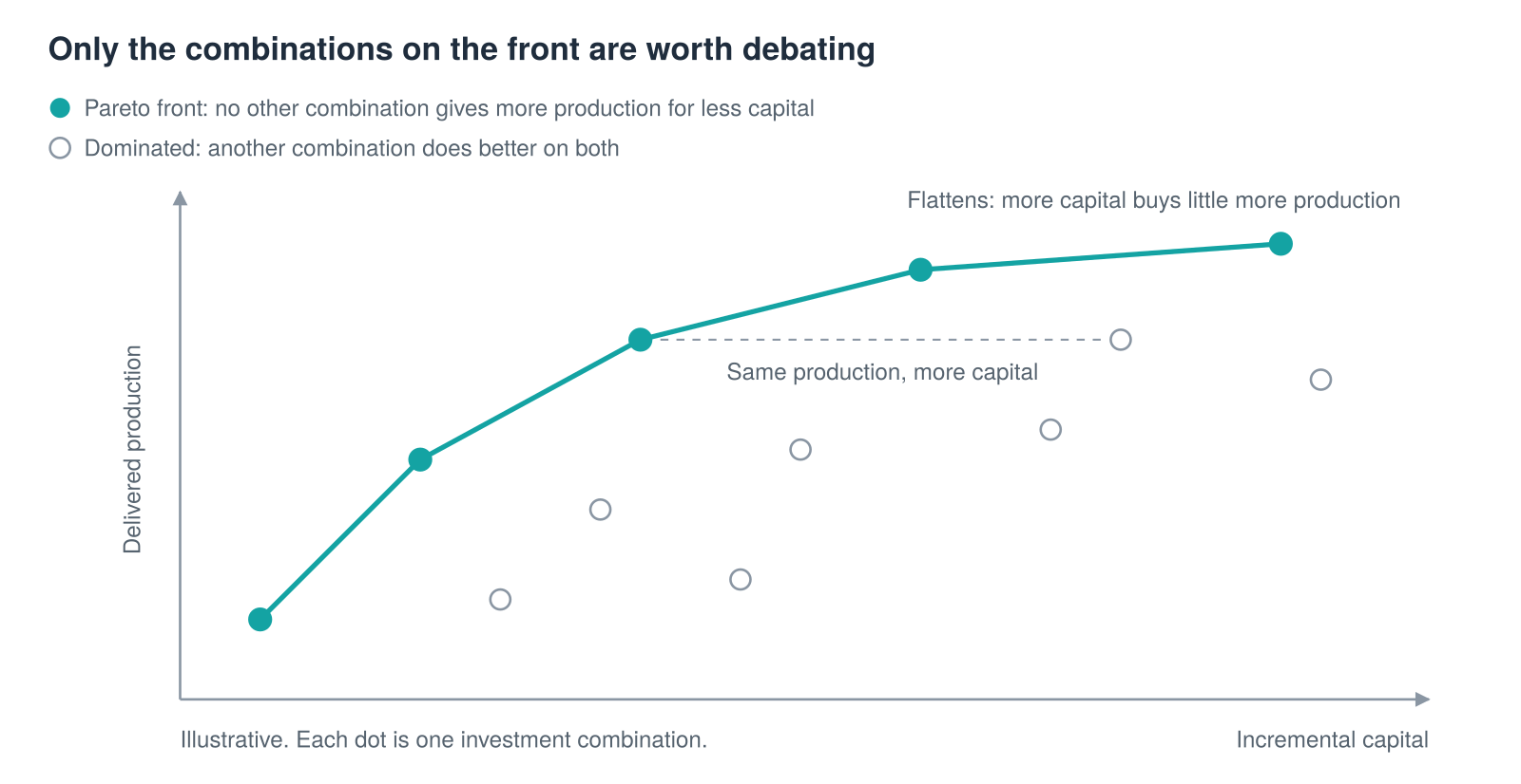
Every combination off the front is beaten on both capital and production by one on it, so the debate narrows to the few on the line.
The front does several useful things.
- It narrows the choice using engineering evidence alone. Two combinations can deliver the same production gain at very different capital. Only one of them belongs on the front.
- It shows where returns diminish. Where the front flattens, the next dollar buys little production. That's often where storage and redundancy proposals sit.
- It fits how capital is actually allocated. Budgets are often fixed. The front shows the best production available at each level of spend.
- It avoids premature aggregation. NPV combines production and capital through price and discount rate assumptions that are themselves uncertain. The front keeps the trade-off visible. NPV then helps choose among a few efficient options, rather than among everything.
The idea extends beyond two objectives. Operating cost, downside production (P10 rather than P50) and production reliability can each be kept as separate objectives. A combination can sit on the front for expected production and well behind it for downside production. Keeping the objectives separate shows that trade-off rather than averaging it away.
But a Pareto front is drawn under a set of assumptions.
Change the operating basis, say lower truck productivity or harder ore, and the front changes shape. Combinations swap places. One that is efficient under the study basis may be dominated under another.
This is the core of many-objective robust decision making (MORDM), developed by Kasprzyk, Nataraj, Reed and Lempert. Find the efficient options under a few deliberately chosen scenarios, including challenging ones. Then re-test them across a wide range of plausible conditions. The options worth taking forward are those that stay on or near the front as the assumptions change.
For mining capital decisions, the set of options is often small enough to evaluate every combination directly, without optimization algorithms. Where it isn't, faster approximation models can screen the space before detailed simulation confirms the short list.
6. Finding where a decision breaks
Rather than testing a handful of familiar optimistic and pessimistic cases, scenario discovery explores many combinations of uncertain conditions and finds the regions where a decision misses its objectives. Bryant and Lempert set out the method.
Suppose a processing expansion is attractive under the expected mine plan. The analysis might show it becomes uneconomic when lower mine productivity combines with reduced equipment availability, leaving the plant short of ore.
That combination is a vulnerability of the investment. The next question is whether it can be addressed.
Would more mining capacity fix it? A different maintenance strategy? Staging the expansion? A change in production sequencing, with no extra capital?
Those alternatives go back through the same tests. The process is iterative:
- Define the investment decision and the performance requirements.
- Identify the important uncertainties and plausible operating conditions.
- Evaluate competing decisions across those conditions.
- Identify where each decision succeeds or fails.
- Develop alternatives that address the most consequential vulnerabilities.
- Re-evaluate the alternatives and their trade-offs.
This is different from selecting a design, forecasting it and checking a few predetermined sensitivities. The analysis is used to discover better decisions.
It also changes the conversation. "The expansion falls short if development rates drop below plan while availability is also low" is something an operations team can judge and act on. A P10 on its own is harder to argue with, and harder to act on.
7. Valuing outcomes when probabilities are uncertain
Expected NPV is a sound metric when outcome probabilities can be estimated credibly. Calculating it needs more than a set of plausible scenarios. It needs a defensible way to weight them.
If the relative likelihoods of several credible operating bases are uncertain, averaging their results doesn't produce a defensible expected NPV. Equal weights can be a useful, stated assumption. They don't establish that the bases are equally likely.
Without reliable probabilities, financial analysis still has a lot to offer. We can:
- Evaluate each investment's NPV across the plausible operating bases.
- Identify the conditions under which an investment misses an economic threshold.
- Compare downside exposure, capital efficiency and the resilience of production.
- Compare regret: how much value each option gives up, in each future, against the best option for that future.
- Test how the ranking changes under different probability assumptions.
Regret fits capital decisions well. Rather than maximizing expected performance, the aim is to limit how much you'd regret the choice in any plausible future.
Rather than concealing uncertainty behind a single expected value, the analysis shows which conclusions depend on uncertain beliefs. It doesn't remove judgment. It makes the basis for it visible.
8. Keeping options open
Major investments involve choices about timing as well as capacity. An operation may eventually need a larger plant, more hoisting, a bigger fleet or more port capacity. Does all of it need to be committed today?
If future performance is uncertain, the ability to expand once better information is available has value. That's the logic of staged investment, real options and adaptive planning. Cardin, de Neufville and Kazakidis showed how designing flexibility into a mining operation can raise its expected value.
At Jansen, integrated modelling supported deferring about $300 million in capital for equipping the second shaft in the initial stage. The capacity wasn't ruled out. The model supported a different decision about when it would be needed.
Deferral isn't free. It can cost production, create construction inefficiencies and expose the operation to future costs. The point is to value flexibility explicitly.
Adaptive planning adds one more step: decide now what evidence would trigger the next investment. For example, sustained plant feed above a set rate, development falling behind plan for two quarters, or a rail service level not being met. Those signposts turn a deferred decision into a planned one.
Sometimes the best decision is to build more. Sometimes it's to invest elsewhere in the operation. And sometimes the most valuable decision is to preserve the option to invest later.
9. A framework for mining decisions
RAND researchers structure these problems with the XLRM framework, set out by Lempert, Popper and Bankes. It maps cleanly onto a mining study:
- X, uncertainties outside the owner's control. Orebody characteristics, workforce and equipment productivity, equipment reliability under a given maintenance strategy, process response, commodity price.
- L, levers the owner controls. Equipment selection, maintenance strategy and resources, infrastructure capacity, redundancy, storage, sequencing, operating strategy, investment timing.
- R, relationships. The operating system linking mining, material handling, processing, storage and logistics. This is what the integrated simulation represents.
- M, measures. Delivered production, production reliability, capital, operating cost, NPV, downside exposure, flexibility.
This separation matters. A value driver isn't necessarily a decision lever. Production is an outcome owners influence through their choices. Price isn't.
Likewise, changing an uncertain assumption isn't the same as changing a design. Crusher reliability shows the difference. More maintenance resources or a standby crusher are levers the owner controls. How much reliability those levers actually buy is still uncertain, and that part is an X.
The framework should answer three questions:
What could happen? Under what conditions? What should we do about it?
10. What simulation can and can't do
Simulation is most valuable when interactions in the operating system drive performance: shared resources, interruptions, inventory, schedules, sequencing and constraints that move over time. These produce nonlinear outcomes that capacity calculations miss.
But simulation alone isn't an uncertainty method. A detailed model can describe operating variability very well while staying anchored to one set of assumptions. Investigating broader uncertainty means explicitly examining alternative assumptions, sometimes alternative model structures, and their consequences for competing decisions.
This approach has practical costs. Detailed models take time to run, and exploring many futures and many options multiplies that. Results with many scenarios and trade-offs are also harder to communicate than a single number.
Both are manageable. Scale the effort to the decision. Evaluate every option where the set is small, screen with faster models where it isn't, and present the few trade-offs that actually matter.
We took this approach at Jansen. Alongside the detailed DICE simulation, a faster static model called SLICE (Simplified Linear Integrated Capacity Estimate) evaluated production capacity for 5,000 combinations of inputs representing risks and uncertainties across mining, hoisting, processing, rail and port (Bouffard and Boggis). The static model estimated capacity far more quickly. The dynamic model was needed to understand the interfaces in the chain (Bouffard).
The objective isn't model complexity or run count.
It's enough understanding of the system and its uncertainty to support a defensible decision.
That also requires transparent assumptions, verification, validation, sound treatment of dependencies and a clear statement of model limitations. A sophisticated result isn't automatically a reliable one.
11. What owners should be accountable for
Owners can't eliminate variability or guarantee production. They can run a disciplined process for testing the assumptions behind their investments.
For many projects, achievable production is among the largest value drivers the owner can influence. A project team should be able to explain its production basis, the evidence behind it, the credible alternatives considered, and what those alternatives mean for the investment.
That goes beyond showing that NPV is sensitive to a production shortfall. It means understanding what might cause the shortfall, how plausible those conditions are, which investments reduce the exposure, and which decisions stay attractive when assumptions change.
For investors, the same information separates a project with a defensible production basis from one whose value rests on a narrow set of optimistic assumptions.
Where probabilities can be estimated credibly, they should inform the valuation. Where they can't, that should be visible, and the investment should be evaluated across the plausible alternatives.
Beyond the forecast
Mining studies are expected to produce forecasts, and they should. Forecasts are essential for design, valuation and capital approval.
But the forecast isn't the decision.
A mining investment commits capital to a physical system whose performance depends on conditions that can't all be known in advance. The challenge isn't only a more precise forecast. It's understanding how the operation performs across plausible conditions, where proposed investments are vulnerable, and which decisions hold their value across those conditions.
The best-supported capital decision isn't necessarily the one with the highest forecast NPV. It's the one whose value, vulnerabilities and trade-offs have been examined.
Understand the range. Value the decisions.
About the author
Bryan Monk, P.Eng., is the founder of MISIM Modelling and has more than 30 years of experience developing simulation models for mining, processing, logistics and complex industrial operations. He is an INFORMS Franz Edelman Laureate and co-author of the published research on BHP's Jansen Potash Project.
References and further reading
- Bonjean Stanton, M. C., and Roelich, K. (2021). Decision making under deep uncertainties: A review of the applicability of methods in practice. Technological Forecasting and Social Change, 171, 120939.
- Bouffard, S. C. (2020). Benefits Realized and Lessons Learned from Modeling the Production Capacity of the Jansen Potash Project. Mineral Processing and Extractive Metallurgy Review, 41(1), 50–58.
- Bouffard, S. C., and Boggis, P. (2019). Stochastic Optimization of the Jansen Potash Production and Logistics Chain. Mineral Processing and Extractive Metallurgy Review, 40(3), 207–217.
- Bouffard, S. C., Boggis, P., Monk, B., Pereira, M., Quan, K., and Fleming, S. (2018). Discrete-Event Simulation Modeling Unlocks Value for the Jansen Potash Project. Interfaces, 48(1), 45–56.
- Bryant, B. P., and Lempert, R. J. (2010). Thinking inside the box: A participatory, computer-assisted approach to scenario discovery. Technological Forecasting and Social Change, 77(1), 34–49.
- Cardin, M.-A., de Neufville, R., and Kazakidis, V. (2008). Process to improve expected value of mining operations. Mining Technology, 117(2), 65–70.
- CIM Mineral Resource & Mineral Reserve Committee (2019). Estimation of Mineral Resources and Mineral Reserves Best Practice Guidelines.
- Dimitrakopoulos, R., Farrelly, C. T., and Godoy, M. (2002). Moving forward from traditional optimization: Grade uncertainty and risk effects in open-pit design. Mining Technology, 111(1), 82–88.
- Kasprzyk, J. R., Nataraj, S., Reed, P. M., and Lempert, R. J. (2013). Many objective robust decision making for complex environmental systems undergoing change. Environmental Modelling & Software, 42, 55–71.
- Lempert, R. J., Popper, S. W., and Bankes, S. C. (2003). Shaping the Next One Hundred Years: New Methods for Quantitative, Long-Term Policy Analysis. RAND Corporation, MR-1626.
- Lempert, R., and Miro, M. Decision-Making Under Deep Uncertainty (DMDU). U.S. Climate Resilience Toolkit, Online Training for Water Utilities.
- Marchau, V. A. W. J., Walker, W. E., Bloemen, P. J. T. M., and Popper, S. W., eds. (2019). Decision Making under Deep Uncertainty: From Theory to Practice. Springer.
- Reddel, M. (2023). Model-Based Policy Analysis under Deep Uncertainty. LessWrong.
- Walker, W. E., Lempert, R. J., and Kwakkel, J. H. (2013). Deep Uncertainty. In Encyclopedia of Operations Research and Management Science, 395–402. Springer.
- MISIM. Transforming the Mine Value Chain: Finding Hidden Capacity and Avoiding Unnecessary Capital.
- MISIM. Variability and uncertainty in mining project studies (video).
